
Hough Transforms with MATLAB’s Image Processing Toolbox
Overview
This tutorial will demonstrate how to find and locate pencils in a given image. The goal is to find the location, angle and length of the pencil(s).
The guide will follow:
- Loading images into MATLAB
- Converting between different colour schemes.
- Edge detection.
- Prepare Image for Hough
- Hough Transforms
- Retrieving information.
NOTE: Look here for the source code.
1 Reading Images
In order to work with images, you fist need to load them into MATLAB. This can be accomplished by using the built in function imread(). This takes a path to an image as input and converts it into a 3D matrix that can be indexed by image(<row>, <col>, <RGB>). With this image variable, we can apply interesting transformations and extract useful information.
img = imread(‘path/to/image/img.jpg’);
imshow(img)
In-order to display the image, we use the function imshow() to print the image to a window (figure). This function also happens to be quite general, as it can display any type of 2D matrix.
2 Colour Schemes
In order to work with the image, we need to first convert it to a color scheme that will best filter out the background from the foreground. A great tool to do this is one of MATLAB's app titled “Color Thresholder”. With this app we can experiment with different color schemes like RGB, HSV, YCbCr and L*a*b in-order-to segment and threshold the image.

Here we used the Color Thresholder app to mask the area surrounding the pencils. The color scheme being used is the YCbCr, and we can adjust the threshold by experimenting with the range sliders that overlay the color histograms to the side.
By utilizing this, we can effectively create a mask to filter out any background noise from the foreground object.
Export the code for the filter by clicking on the “Export” button.
%% Convert RGB image to LAB
    RGB = im2double(img);
    cform = makecform('srgb2lab', 'AdaptedWhitePoint', whitepoint('D65'));
    I = applycform(RGB,cform);

    channel1Min = 13.262;
    channel1Max = 67.444;

    % Define thresholds for channel 2 based on histogram settings
    channel2Min = -1.205;
    channel2Max = 14.341;

    % Define thresholds for channel 3 based on histogram settings
    channel3Min = -13.473;
    channel3Max = 13.090;

    % Create mask based on chosen histogram thresholds
    BW = (I(:,:,1) >= channel1Min ) & (I(:,:,1) <= channel1Max) & ...
        (I(:,:,2) >= channel2Min ) & (I(:,:,2) <= channel2Max) & ...
        (I(:,:,3) >= channel3Min ) & (I(:,:,3) <= channel3Max);

    % Invert mask
    BW = ~BW;

    % Initialize output masked image based on input image.
    maskedRGBImage = RGB;

    % Set background pixels where BW is false to zero.
    maskedRGBImage(repmat(~BW,[1 1 3])) = 0;
4 Edge Detection
Now that we have a masked image, this is when the fun really starts.
We first convert the image to Gray scale by using the function rgb2gray(). We then apply the edge() function onto the gray scale image to find all the outline edges.
Edge(): Takes in two parameters, one being the image to perform the convolution on, and (2) a string value dictating the type of edge detection.
%% Find the edges of the image using laplacian of gaussian.
imgedg = edge(maskedGray, 'log');
imshow(imgedg)

<method> := 'canny', 'log', 'sobel', ...
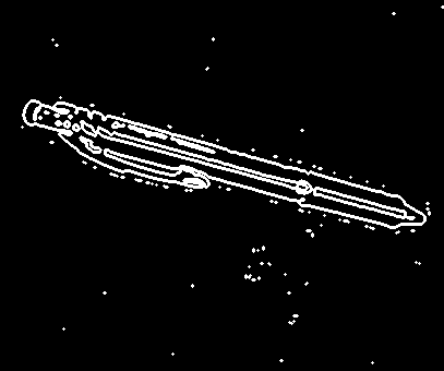
Here we are using the 'log' method to detect the edges. This will use the Laplacian of Gaussian through a convolution mask and find the gradient of the gradient on the 2D plane producing an outline of the object.
Next step is to smooth out the image and thicken up the edge lines. Use the imdilate() method to perform this and you should produce something similar to the image on the right.
smooth = imdilate(imgedg, strel('disk',1));
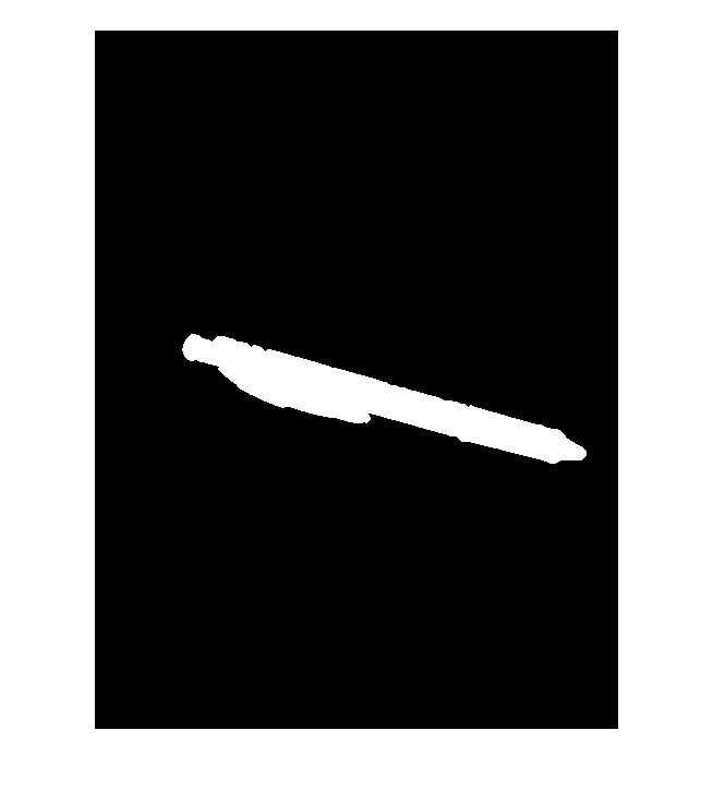
With the smooth image, we can clean up the noise by using bwboundaries(), imclearborder(), and bwareaopen() consecutively one after the other. This will convert the edges into defined blobs and we can then clean up and bwareaopen() will remove all blobs smaller than a predefined size—in this particular case we will use a size of 400 px, which will remove blobs that contain less than 400 pixels.
%% Find Regions and display
[B, L] = bwboundaries(smooth, 'holes');

%% Clean the border of the image from artifacts.
L = imclearborder(L);

%% Clean up image based on segments
L = bwareaopen(L, 400);
This will result in the following two images

5 Prepare Image for Hough Transforms
Now that we have a blob representation of the pencil, we need to erode it to obtain a skeletal like representation of blob. This can be accomplished with the bwmorp() function.
This function allows you to perform morphological transforms onto the image by eroding away at the pixels from the outside in. The result is a skeletal like structure and to obtain this, we pass in the parameter 'thin'.
%% Thin the image
L_thin = bwmorph(L, 'thin', inf);

'thin' =  It removes pixels so that an object without holes shrinks to a
minimally connected stroke, and an object with holes shrinks to a connected
ring halfway between each hole and the outer boundary.
This will thin the object to a line representation for the blob. As can be seen on the left, the blob representation of the pencil is now composed of a tree like structure.
Next is to transform the skeletal image with Hough.
Hough(<image>), takes in an image as a parameter and produces H, theta, and rho as output.
%% Compute hough transform.
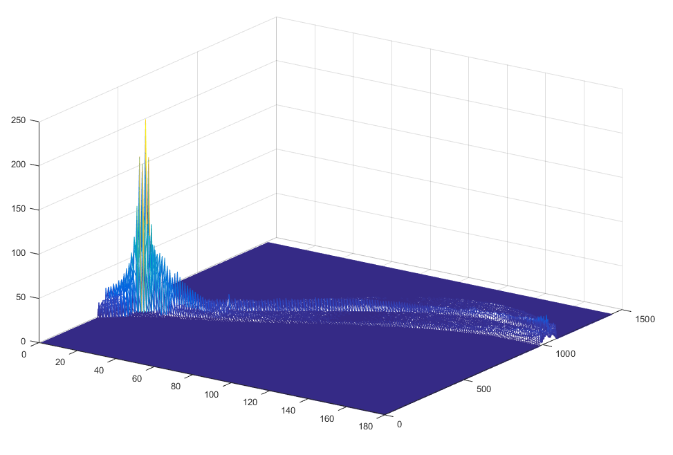
[H, theta, rho] = hough(L_smooth);This works by iteratively taking each pixel and transforming them into a histogram like two-dimensional representation called the Hough Space. All the Hough Spaces for all the pixels are summed together in a voting procedure where the global maximum on the Hough Plane is where the line is most likely to be. This plane can be seen on the right, the peak is the most likely common line. The angle theta (x-axis) and distance rho (y-axis) are plotted on the bottom.
This Hough plane (H), can then be passed into the function houghpeaks(<H>, <# of peaks to find>, <params>, …), where we can locate these maximums in the plane.
%% Find peaks in teh Hough transform
peaks = houghpeaks(H, 6, 'threshold', 10);
Here, 'threshold', represents the minimum value to be considered a peak.
Finally, to get the lines that best fit the image we have transformed, we need to pass in peaks, theta, rho, and image variables into the function houghlines().
%% Find lines using houghlines
lines = houghlines(L_smooth, theta, rho, peaks, 'FillGap', 200, 'MinLength', 200);
With the new variable lines, which holds all the line information inside a structure, we can print the information back onto the original image.
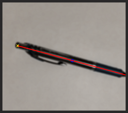
xy = [lines.point1; lines.point2];
plot(xy(:, 1), xy(:,2), 'Linewidth', 2, 'Color', 'green');
This will print the lines onto the original image as as seen below.
This wraps up the quick tutorial on Hough and the image processing toolbox. If you have questions, concerns, or criticism be sure to leave a comment.